
A face recognition system can identify a person without training a large convolutional network from scratch. This project converts each portrait into a 2,622-value VGG-Face descriptor, compresses those features with PCA, and maps the result to one of 100 identities with an RBF support vector machine. The completed notebook also identifies two held-out portraits of Benedict Cumberbatch and Dwayne Johnson correctly.
The interesting work sits between loading an image and printing a name. A 10,770-image archive puts file paths under real strain. OpenCV color channels need correcting. Training statistics have to stay out of the test set, and inference must repeat the same transformations in the same order. This case study follows those decisions and explains what the final outputs prove.
What Does This Face Recognition Pipeline Do?
The pipeline performs closed-set face identification across 100 known people. It assumes the face is already visible and reasonably aligned, extracts a numerical descriptor with a pretrained VGG-Face network, and classifies that descriptor with an SVM.
| Stage | Input | Operation | Output |
|---|---|---|---|
| Dataset indexing | PINS folders | Read identity and filename metadata | One record per portrait |
| Image preparation | JPEG portrait | Convert BGR to RGB, normalize, resize | Model-ready image array |
| Feature extraction | Prepared face | Run the pretrained VGG-Face descriptor | 2,622 numerical features |
| Feature scaling | Raw descriptor | Fit StandardScaler on training data | Centered, scaled features |
| Compression | Scaled features | Retain the main PCA directions | Lower-dimensional vector |
| Classification | PCA vector | Apply an RBF SVM | Encoded identity label |
| Interpretation | Encoded label | Apply LabelEncoder.inverse_transform | Folder-style person name |
This is face recognition, not face detection. Detection answers, “Where is a face?” Recognition answers, “Which enrolled identity does this face resemble?” The assignment’s earlier sections use masks and Haar cascades for location. This section begins with aligned portraits and concentrates on identity.
How Is the PINS Dataset Turned Into Usable Metadata?
The dataset becomes manageable when every file is represented by three values: its base directory, identity folder, and filename. The project stores those values in a small IdentityMetadata class instead of loading all image pixels into memory at once.
class IdentityMetadata:
    def __init__(self, base, name, file):
        self.base = base
        self.name = name
        self.file = file

    def image_path(self):
        return os.path.join(self.base, self.name, self.file)
The class does little. A record can rebuild the path whenever an image is needed, and it keeps the identity label next to the file that produced it.
The loader walks through each identity directory and accepts .jpg and .jpeg files:
def load_metadata(path):
    metadata = []
    for identity in os.listdir(path):
        identity_path = os.path.join(path, identity)
        for filename in os.listdir(identity_path):
            extension = os.path.splitext(filename)[1].lower()
            if extension in {'.jpg', '.jpeg'}:
                metadata.append(
                    IdentityMetadata(path, identity, filename)
                )
    return np.array(metadata)
Labels come straight from directory names such as pins_Benedict Cumberbatch, and one broken image can be isolated without losing the rest of the dataset.
Archive paths deserve an explicit check
The notebook catches an extraction error involving a Windows path and a folder name with spaces. That output is useful evidence about the archive. Large image archives often contain mixed separators, trailing spaces, macOS metadata folders, or filenames that fail on another operating system.
A stronger loader checks os.path.isdir(identity_path) before entering a directory, normalizes extensions with .lower(), and records failed paths in a list. Silent except: blocks keep a long embedding run alive, but they hide the cause. Logging the filename and exception makes the run auditable.
Why Does OpenCV Color Conversion Matter?
OpenCV reads a normal color image in BGR order, while Matplotlib and most RGB-trained neural-network workflows expect RGB order. The project corrects that difference inside one reusable function:
def load_image(path):
    image = cv2.imread(path)
    if image is None:
        raise ValueError(f"Could not read image: {path}")
    return cv2.cvtColor(image, cv2.COLOR_BGR2RGB)
Without the conversion, blue and red channels exchange places. The portrait may still look face-like, so the error is easy to miss, but the descriptor receives a color distribution different from the one the workflow intends.
The image is then converted to float32, divided by 255, and resized. OpenCV documents cv.resize as the operation that changes an image to an explicit output size, while its color-conversion API defines the BGR and RGB transformations used here.
The syntax matters less than one rule: training and inference must apply identical image preparation. If dataset portraits enter the descriptor at 224 x 224 pixels, test portraits belong at 224 x 224 as well. A separate 300 x 300 copy can be created for display, but it must not replace the model input.
How Does VGG-Face Produce a 2,622-Value Descriptor?
VGG-Face supplies the pretrained visual representation in this project. The network contains five convolutional blocks followed by larger convolutional layers and a final 2,622-class output. The notebook loads pretrained weights and creates a second Keras model whose output stops immediately before softmax.
model = vgg_face()
model.load_weights('vgg_face_weights.h5')

vgg_face_descriptor = Model(
    inputs=model.layers[0].input,
    outputs=model.layers[-2].output
)
The resulting vector has shape (2622,) for a 224 x 224 input. Each value is part of the representation learned by the network. The SVM receives this vector rather than the original 150,528 RGB values in a 224 x 224 x 3 image.
The Oxford Visual Geometry Group introduced VGG-Face in the 2015 Deep Face Recognition paper. Its training work used 2.6 million images across more than 2,600 identities. The transfer-learning idea is simple: a model trained to separate many faces can act as a feature extractor for a smaller classification problem. Keras describes this pattern as running data through a pretrained base model once, storing the outputs, and training a smaller model on those extracted features.
The notebook uses the pre-softmax output as its embedding
The word “embedding” can refer to outputs from different network layers. In this notebook, it means the flattened 2,622-value layer immediately before softmax. Other VGG-Face implementations use a 4,096-value fully connected layer or normalize descriptors before comparing them. Naming the exact layer prevents two implementations from claiming to use the same embedding while producing incompatible vectors.
Failed image reads receive a zero vector
The embedding matrix is allocated in advance:
embeddings = np.zeros((metadata.shape[0], 2622))

for index, item in enumerate(metadata):
    try:
        image = prepare_for_vgg(item.image_path())
        batch = np.expand_dims(image, axis=0)
        embeddings[index] = vgg_face_descriptor.predict(batch)[0]
    except Exception as error:
        failed_images.append((item.image_path(), str(error)))
Preallocation fixes the matrix shape even when one image fails. A zero descriptor is acceptable as an assignment fallback, but a production pipeline needs a second step: remove failed rows and their labels before training. Otherwise, several unreadable images create identical zero points that carry unrelated identity labels.
Do Squared L2 Distances Separate Similar and Different Faces?
Squared L2 distance provides a quick diagnostic before classification. The notebook compares selected pairs of descriptors using the sum of squared feature differences:
def squared_l2_distance(first, second):
    return np.sum(np.square(first - second))
Two portraits of the same person are expected to sit closer in descriptor space than portraits of different people. The paired-image plots make this relationship visible by placing two faces beside the numerical distance.
Distance checks catch pipeline mistakes early. Near-identical values for every pair may indicate repeated zero vectors. Unstable values may point to inconsistent normalization, color conversion, cropping, or input size. A classifier can hide these problems by fitting the labels anyway; pairwise inspection exposes them before PCA and SVM add more machinery.
Squared distance is not a calibrated identity threshold. Its magnitude depends on the descriptor layer, preprocessing, and dataset. A real verification system estimates a threshold on validation pairs and reports false-match and false-non-match rates.
How Are Training and Test Data Kept Separate?
The notebook assigns every ninth metadata record to the test set and uses the other eight records for training. That produces an approximate 8:1 split while distributing regularly positioned images across both partitions.
indices = np.arange(metadata.shape[0])
train_idx = indices % 9 != 0
test_idx = indices % 9 == 0

X_train = embeddings[train_idx]
X_test = embeddings[test_idx]
y_train = labels[train_idx]
y_test = labels[test_idx]
The labels are encoded as integers with LabelEncoder. More importantly, both StandardScaler and PCA are fitted only on X_train. The test set receives .transform() calls using statistics learned from the training set.
encoder = LabelEncoder()
y_train_encoded = encoder.fit_transform(y_train)
y_test_encoded = encoder.transform(y_test)

scaler = StandardScaler()
X_train_scaled = scaler.fit_transform(X_train)
X_test_scaled = scaler.transform(X_test)
Fitting the scaler on all 10,770 descriptors would leak test-set means and variances into training. The same rule applies to PCA. A preprocessing step learns from data whenever it estimates a mean, variance, component direction, vocabulary, or threshold.
For a repeatable extension, use a stratified split with a fixed random state and verify that all 100 identities appear in both partitions. For a harder evaluation, group near-duplicate photos or capture sessions so closely related images cannot land on both sides.
Why Apply StandardScaler Before PCA and an RBF SVM?
Standardization stops high-variance descriptor coordinates from dominating PCA and the RBF distance calculation. StandardScaler subtracts each training-feature mean and divides by its training standard deviation, then reuses those values for test and inference data.
The scikit-learn documentation notes that RBF SVM objectives can behave poorly when feature variances differ by orders of magnitude. Scaling makes the numerical contribution of each descriptor coordinate more comparable.
The order is deliberate:
Fit the scaler on training embeddings.
Transform training and test embeddings.
Fit PCA on scaled training embeddings.
Transform both partitions with the fitted PCA object.
Train the SVM on the PCA representation.
Changing this order changes the geometry of the problem.
How Does PCA Reduce the Face Descriptor?
PCA projects the 2,622 scaled features onto a smaller set of directions that explain most of the training variance. The notebook computes the covariance matrix, eigenvalues, and cumulative explained variance manually. The first index crossing 95 percent is reported as 123.
That output tells us the descriptor contains substantial redundancy. Thousands of coordinates can be compressed to roughly one hundred principal directions before classification.
There is a small indexing detail worth fixing. An index of 123 refers to the 124th component because Python counts from zero. Passing n_components=123 retains 123 components, which may fall slightly below the inspected threshold. Scikit-learn already supports the intended rule directly:
pca = PCA(
    n_components=0.95,
    svd_solver='full',
    whiten=True,
    random_state=2022
)

X_train_pca = pca.fit_transform(X_train_scaled)
X_test_pca = pca.transform(X_test_scaled)
With n_components=0.95 and the full solver, PCA selects the count required to exceed the requested explained-variance proportion. This removes the off-by-one ambiguity and exposes the chosen value through pca.n_components_.
Whitening rescales retained components to unit variance. That can help an RBF classifier when the leading components otherwise dominate, but it also removes relative variance information. The choice belongs in cross-validation rather than being treated as universally better.
How Is the RBF SVM Configured?
The classifier uses an RBF kernel with C=1, gamma=0.001, balanced class weights, and a fixed random state. The RBF kernel lets the decision boundary curve through the PCA feature space instead of forcing a linear separation.
classifier = SVC(
    C=1,
    gamma=0.001,
    kernel='rbf',
    class_weight='balanced',
    random_state=2022
)

classifier.fit(X_train_pca, y_train_encoded)
Scikit-learn handles multiclass SVC through a one-vs-one scheme. With 100 identities, the model learns pairwise class boundaries internally. Balanced class weights reduce the effect of unequal image counts across identity folders.
The notebook prints a score of 1.0 on X_train_pca. That means every training descriptor is classified correctly. It does not establish 100 percent accuracy on unseen faces. RBF SVMs can fit a training set very closely, especially after a high-capacity embedding model has already separated the classes.
A defensible evaluation also reports the test score, macro F1, per-class recall, and a confusion matrix. Cross-validation can tune C, gamma, PCA whitening, and the variance threshold without using the final test set for repeated decisions.
How Are New Portraits Classified?
Inference repeats the fitted pipeline in the original order. The test portrait is loaded, converted to RGB, normalized, resized to 224 x 224, passed through VGG-Face, scaled, projected with PCA, and classified by the SVM.
def predict_identity(path):
    image = load_image(path)
    display_image = cv2.resize(image, (300, 300))

    model_image = cv2.resize(image, (224, 224))
    model_image = (model_image / 255.0).astype(np.float32)

    descriptor = vgg_face_descriptor.predict(
        np.expand_dims(model_image, axis=0),
        verbose=0
    )[0]

    scaled = scaler.transform(descriptor.reshape(1, -1))
    reduced = pca.transform(scaled)
    encoded_prediction = classifier.predict(reduced)
    name = encoder.inverse_transform(encoded_prediction)[0]

    return name, display_image
The solution’s final figures identify the first portrait as pins_Benedict Cumberbatch and the second as pins_Dwayne Johnson. These two results confirm that the saved preprocessing objects and classifier can produce sensible labels for the supplied portraits.
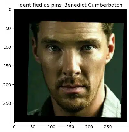
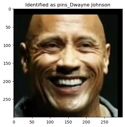
The test is small but concrete. It is stronger than showing training accuracy alone because the two input files sit outside the descriptor matrix used to fit the classifier. It is still weaker than a measured test-set evaluation across all 100 classes.
What Do the Results Prove and What Remains Unmeasured?
The notebook proves that the end-to-end data path works for the supplied examples. It does not yet prove deployment-grade accuracy, open-set recognition, or demographic parity.
| Observed result | Supported interpretation | Unsupported interpretation |
|---|---|---|
| Descriptor shape is (2622,) | The selected VGG-Face layer produced the expected feature length | Every image produced a useful descriptor |
| PCA threshold crosses near index 123 | The scaled features can be reduced substantially | Exactly 95 percent variance was retained by n_components=123 |
| Training score is 1.0 | The SVM fits the training representation | Test accuracy is 100 percent |
| Both supplied portraits receive correct labels | The inference chain works for these 2 known identities | Unknown people are rejected correctly |
In a student report, stating a limitation precisely shows that the author can tell a demonstration from an evaluation.
Six Improvements That Make the Project Easier to Defend
The notebook already works. These six changes make its results easier to trust.
1. Use one preprocessing function everywhere
Create one function for RGB conversion, normalization, and 224 x 224 model resizing. Call it during batch embedding and single-image inference. This removes silent training-serving skew.
2. Use a scikit-learn Pipeline
Combine StandardScaler, PCA, and SVC in one fitted Pipeline. A pipeline prevents transforms from being applied in the wrong order and makes cross-validation safer.
from sklearn.pipeline import Pipeline

face_model = Pipeline([
    ('scale', StandardScaler()),
    ('pca', PCA(n_components=0.95, whiten=True,
                svd_solver='full', random_state=2022)),
    ('svm', SVC(kernel='rbf', C=1, gamma=0.001,
                class_weight='balanced'))
])
3. Report test metrics
Print test accuracy and macro F1, then inspect a confusion matrix. Accuracy answers how often the model is right overall. Macro F1 gives each identity equal weight even when folder sizes differ.
4. Record failed files instead of hiding them
Store the path and exception for every unreadable image. Remove those rows from both embeddings and labels before fitting. The final report can state exactly how many of 10,770 files were usable.
5. Add an unknown-person decision
The present SVM is closed-set. It always chooses one of the 100 enrolled identities, even for a person who never appears in PINS. A practical recognizer needs a rejection rule based on calibrated confidence or distance to known classes.
6. Separate identification from responsible deployment
Classroom success on aligned celebrity portraits does not authorize use for attendance, surveillance, access control, or law enforcement. The Oxford VGG-Face dataset page warns that its identity distribution may not represent the global population. NIST evaluations have also documented demographic differences in false-positive and false-negative behavior across face-recognition algorithms.
Common Errors in a VGG-Face, PCA and SVM Assignment
Most failures occur at the boundaries between components rather than inside the SVM.
BGR images appear with wrong colors: convert OpenCV output to RGB before plotting or using an RGB workflow.
The descriptor shape changes: keep the model input at the size used to create the training embeddings.
PCA rejects the matrix: fit the scaler and PCA on a two-dimensional array shaped as samples by features.
Test labels cause an encoder error: verify every test identity exists in the encoder fitted on training labels.
Results change between runs: sort directory listings and use explicit random states.
Training accuracy looks perfect: compute metrics on data excluded from all fitting and tuning.
An unknown face gets a confident name: add rejection logic because a closed-set SVM cannot answer “none of the above.”
Memory use spikes during extraction: process images sequentially and store only descriptors, not every decoded image.
Students working through a large notebook can use How to Tackle a Large Programming Assignment Step by Step to separate data loading, feature extraction, evaluation, and reporting into testable checkpoints. The same discipline makes computer-vision bugs easier to locate.
A Submission Checklist for This Face Recognition Project
Before exporting the notebook, verify these 14 items:
Confirm the PINS archive extracts into identity folders.
Remove non-image folders such as __MACOSX from metadata traversal.
Log every unreadable image path.
Convert BGR images to RGB.
Use the same normalization and model size for training and inference.
Confirm every stored descriptor has 2,622 values.
Remove failed zero-vector rows before training.
Fit LabelEncoder, StandardScaler, and PCA with training data only.
Record pca.n_components_ and explained variance.
Report both training and test metrics.
Display same-identity and different-identity distance pairs.
Show the two supplied test portraits with predicted labels.
Run all notebook cells in order and retain their outputs.
Explain the closed-set and dataset-bias limitations in plain language.
The Why Testing Matters in Programming Assignments guide explains why visible output is not enough when preprocessing and evaluation can fail silently. For a broader view of where this project fits, see 12 Common Programming Assignments and How to Approach Them.
Students who want a line-by-line explanation of their own notebook can use Python Homework Help to work with a human specialist. Check the course’s collaboration policy, disclose outside assistance when required, and understand every step you submit.
Frequently Asked Questions
Is VGG-Face the classifier in this project?
No. VGG-Face extracts a numerical descriptor from each portrait. PCA compresses the descriptor, and the SVM maps the compressed vector to one of the 100 identity labels.
Why use an SVM after a neural network?
The pretrained neural network already supplies features that separate facial identities. An SVM can learn the smaller course-specific label set without retraining the full convolutional model.
Why is StandardScaler fitted before PCA?
Scaling prevents high-variance descriptor coordinates from dominating the principal directions and RBF distances. The scaler is fitted on training data and reused unchanged for test portraits.
Does a training score of 1.0 mean the model is perfect?
No. It means the classifier labels its training samples correctly. Generalization requires metrics from excluded test data, preferably supported by cross-validation and per-class results.
Why did PCA select about 123 components?
The cumulative eigenvalue calculation crossed the 95 percent threshold near index 123. The exact retained count depends on zero-based indexing and the PCA configuration. Passing n_components=0.95 lets scikit-learn select the count directly.
Can this model recognize anyone?
No. The classifier chooses among identities present in its training labels. Recognizing an unknown person requires a rejection threshold and validation data that includes non-enrolled identities.
Why must test portraits use the same input size?
The descriptor layer expects the same spatial pipeline used for training embeddings. A different size can change the output shape or representation, which then conflicts with the fitted scaler and PCA objects.
Is this workflow suitable for real biometric decisions?
No. It is an educational closed-set classifier built from aligned celebrity images. A real biometric system needs consent, security controls, representative evaluation data, calibrated thresholds, error analysis, and legal review.